A shared operating lens for teams navigating schedules that no longer behave exceptionally

We analyzed 9,581 vessel schedules and 89,208 schedule change events. The pattern is not cyclical. It’s baseline.

I. The Cargo Receiving Window - The Boundary That Actually Matters

For exporters, the critical operational constraint is not vessel arrival.

It is the Cargo Receiving Window (CRW).

The Cargo Receiving Window is the period between:

• ERD (Earliest Return Date) - when the terminal begins accepting containers
• CY Cut (Container Yard Cutoff) - when the terminal stops accepting them

It is the time between:

“You may bring it”
and
“You are too late.”

If the CRW moves:

• Gate appointments must shift
• Drayage must be rescheduled
• Documentation must be revisited
• Customer timelines must be updated

This is the boundary operators actually manage.

Figure 1 - THE CARGO RECEIVING WINDOW

Vessel arrival matters. Rate volatility matters. But the CRW determines whether a container can physically be delivered.

Everything in this article flows from that boundary.

II. Structural Volatility - Per 100 Shipments

Across 9,581 vessel schedules and 89,208 schedule change events , a consistent pattern emerges.

Figure 2 - Per 100 Shipments: Structural Load

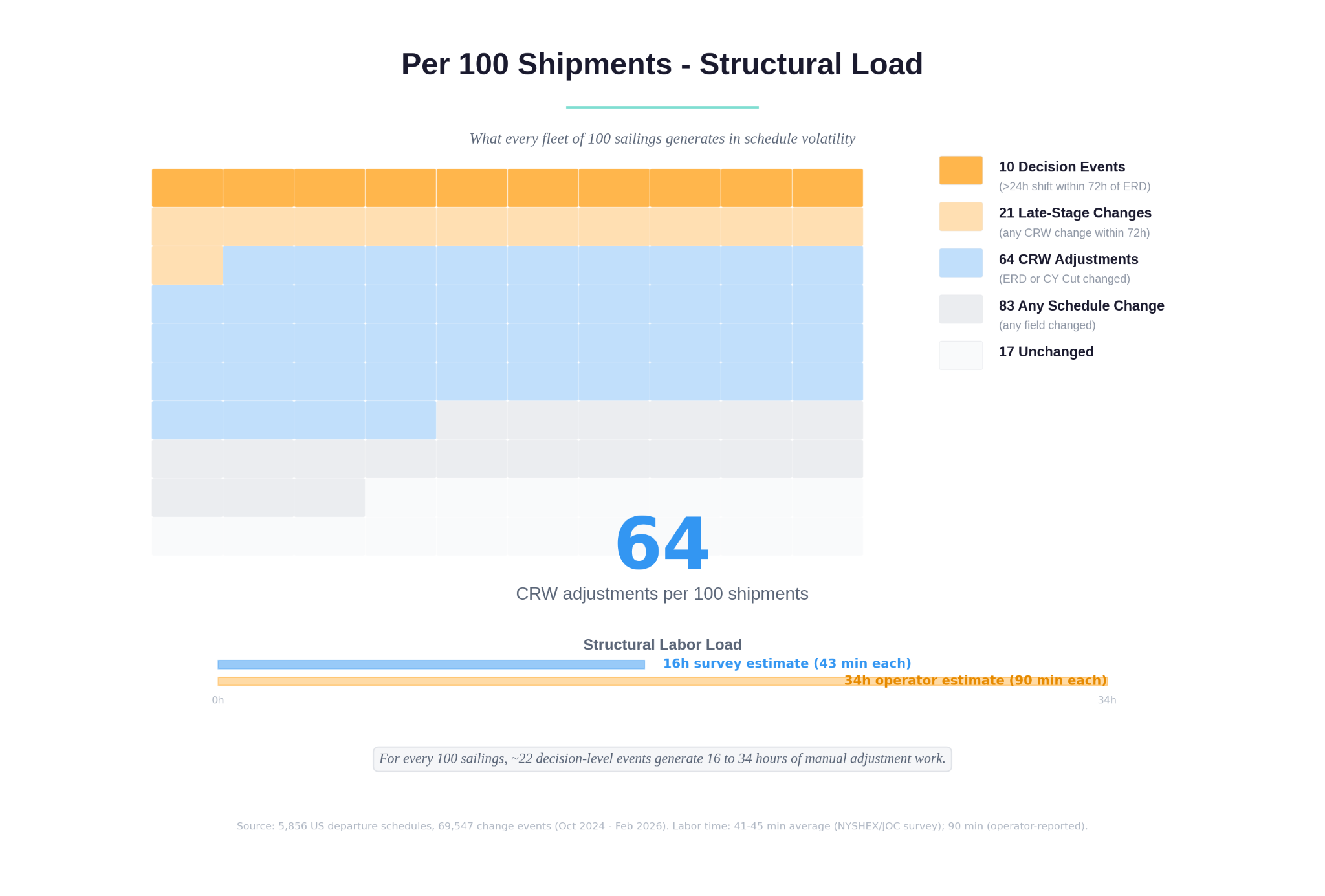
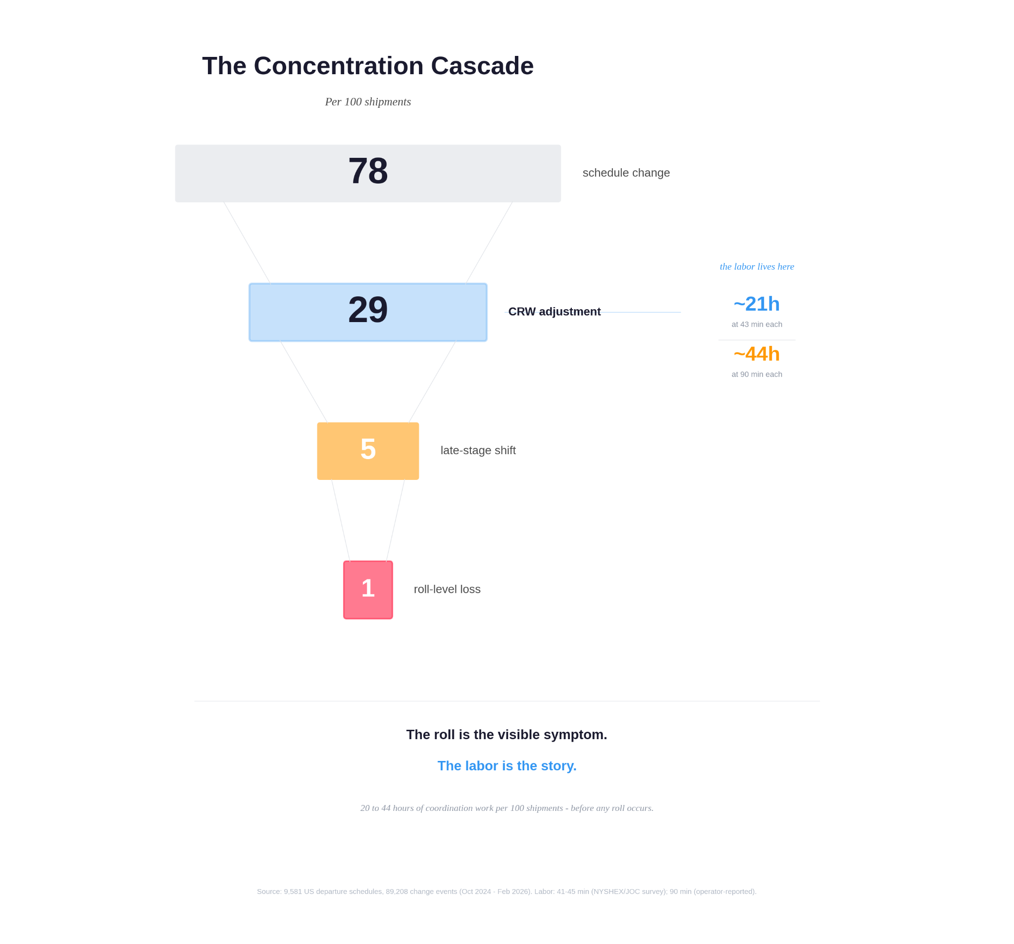
Out of every 100 export shipments:

• 78 will experience at least one schedule change
• 29 will experience a change affecting the CRW - an operational disruption
• 5 will experience a CRW change inside the final 72 hours before ERD

If we stop there, the story sounds manageable.

It is not.

Structural volatility is a workload problem - and when compression intensifies, a roll problem too.

Not all rolls are catastrophic. Many are recoverable.

But every roll begins as compression. And every compression begins as adjustment.

Those 29 CRW adjustments are not alerts.

They are conversations, rebookings, calendar resets, documentation updates, and phone calls.

The labor lives in the 29.

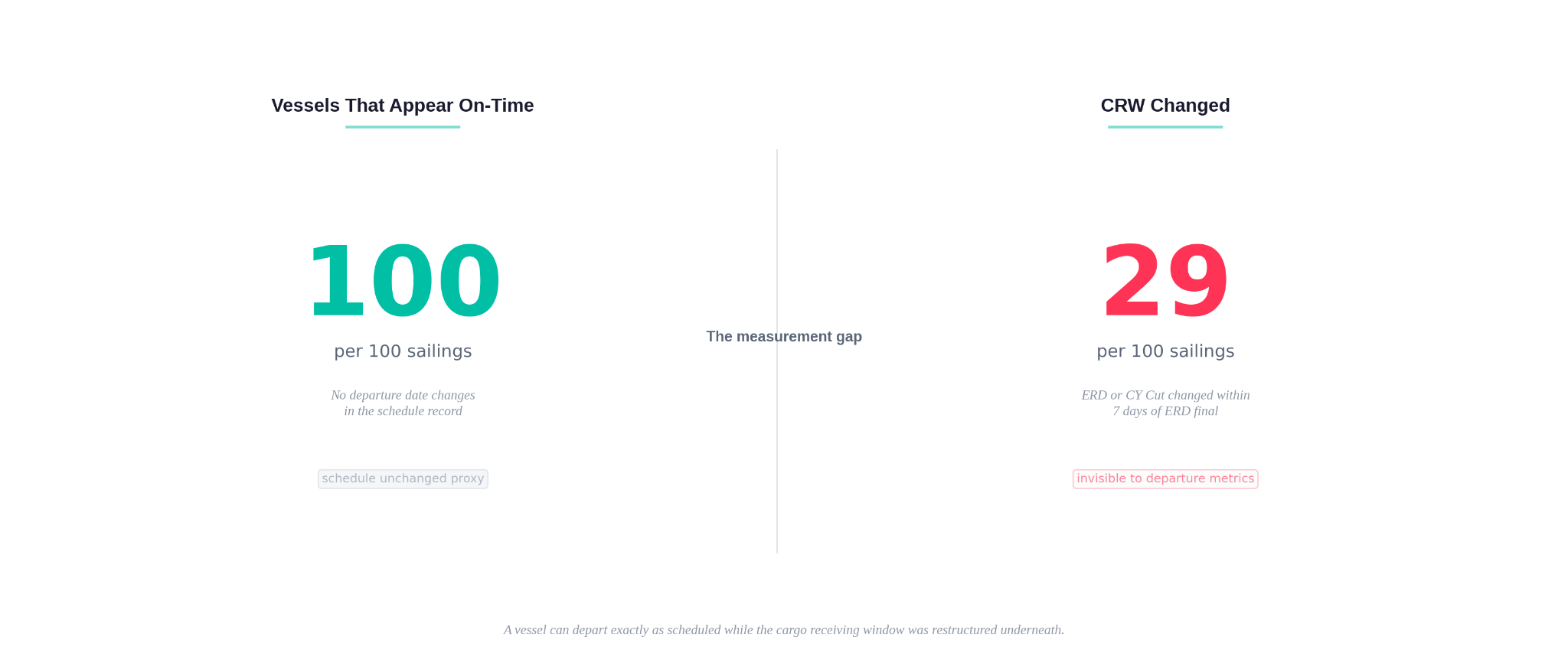
Figure 3 - The Measurement Gap

III. The Time Tax - Where Structural Volatility Actually Hurts

According to the 2023 Vessel Schedule Impact Report, respondents spend 41 to 45 minutes, on average, adjusting a shipment due to an ERD change (see page 14).

That survey was completed primarily by managers and directors.

When this timing was shared with frontline coordinators - the people doing the work - many reported the real figure is closer to 90 minutes.

Now apply that to 100 shipments.

Figure 4 - Structural Adjustment Load at Dataset Scale

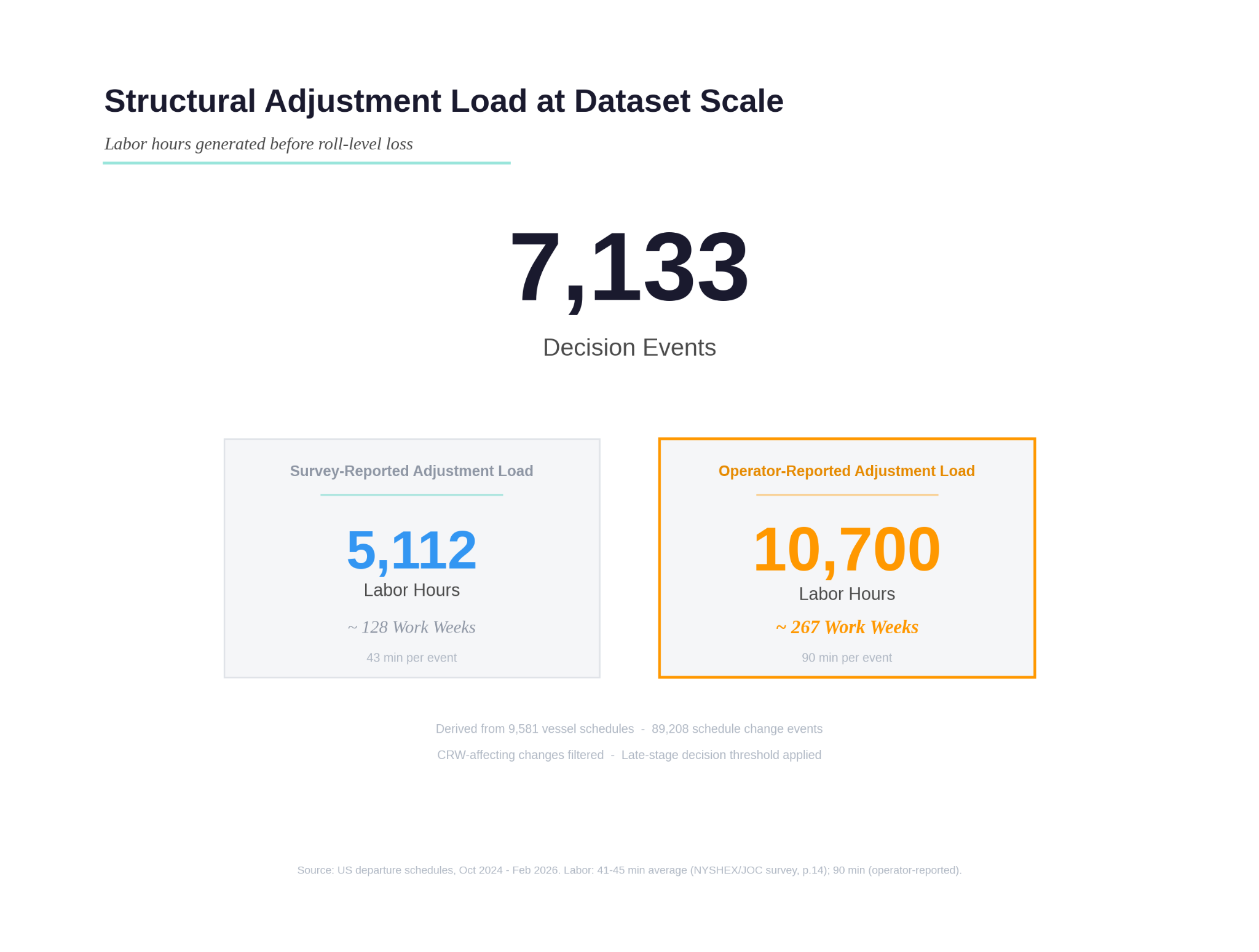
Out of 100 shipments:

• 29 require CRW-related adjustment
• At 43 minutes each, that equals roughly 20-22 labor hours
• At 90 minutes each, that equals roughly 43-44 labor hours

That is half to a full work week of coordination time per 100 shipments.

Before any roll occurs.

Across the full dataset, those 7,117 decision events translate into thousands of labor hours - before we even discuss financial loss.

Structural volatility rarely explodes.

It accumulates.

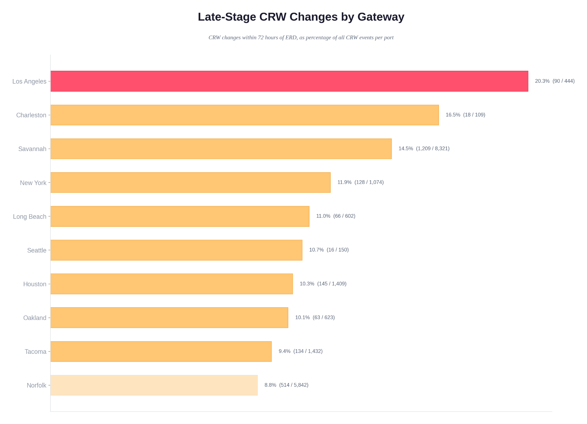
IV. Where 5 Concentrate - The 72-Hour Zone

Of the 29 shipments requiring CRW adjustment:

~5 per 100 will move inside the final 72 hours before ERD.

This is where planning space collapses.

Late-stage change is not merely a timing inconvenience. It is when:

• Drayage is already booked
• Appointments are locked
• Production is committed

In the collapse example shown, a 19-day drift eliminated roughly two-thirds of the original actionable window before the first alert.

The shipment did not fail immediately.

It lost planning space first.

Figure 5 - Anatomy of a Window Collapse

Inside the 72-hour boundary, recovery options narrow sharply.

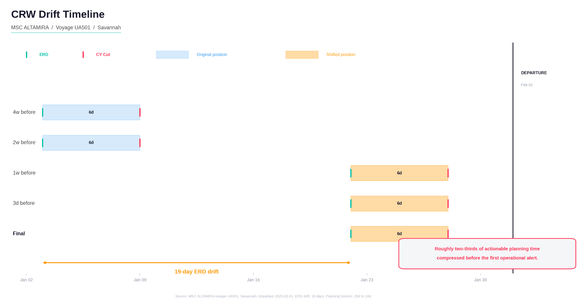
Figure 6 - Late-Stage CRW Changes per 100 by Gateway

Of those 5 late-stage shipments: ~1 per 100 will escalate into a roll-level loss.

But that 1 sits on top of the 29 adjustments that preceded it.

The roll is the visible symptom.

The compression is the mechanism.

V. Structural Volatility Is Uneven - And It Multiplies the Time Tax

The “1 per 100” figure reflects the aggregate dataset across all corridors.

At specific gateways, roll-level exposure can be materially higher.

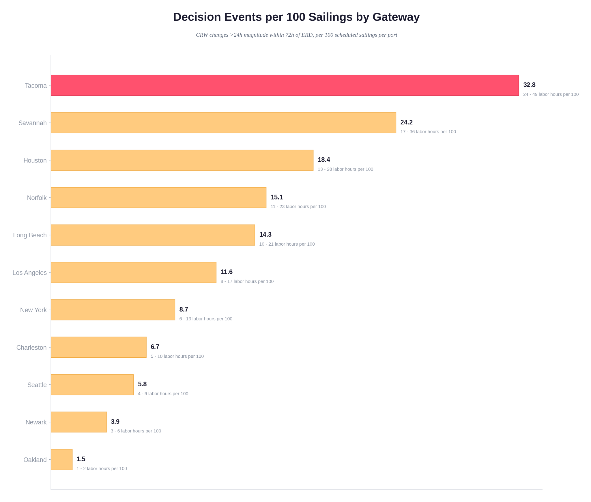
Per 100 sailings:

• Long Beach → ~48 roll-level disruptions
• Seattle → ~47
• Savannah → ~39
• Houston → ~19
• Oakland → ~16

In a high-volatility corridor:

100 shipments may produce 40 roll-level disruptions.

At 43 minutes per adjustment, that is ~30 labor hours.
At 90 minutes, ~60 hours.

Structural volatility is not just about the rare collapse.

It is about corridor-specific workload concentration.

Two exporters moving identical volumes through different gateways may operate under completely different adjustment burdens.

Figure 7 - Corridor Variation + Carrier Spread

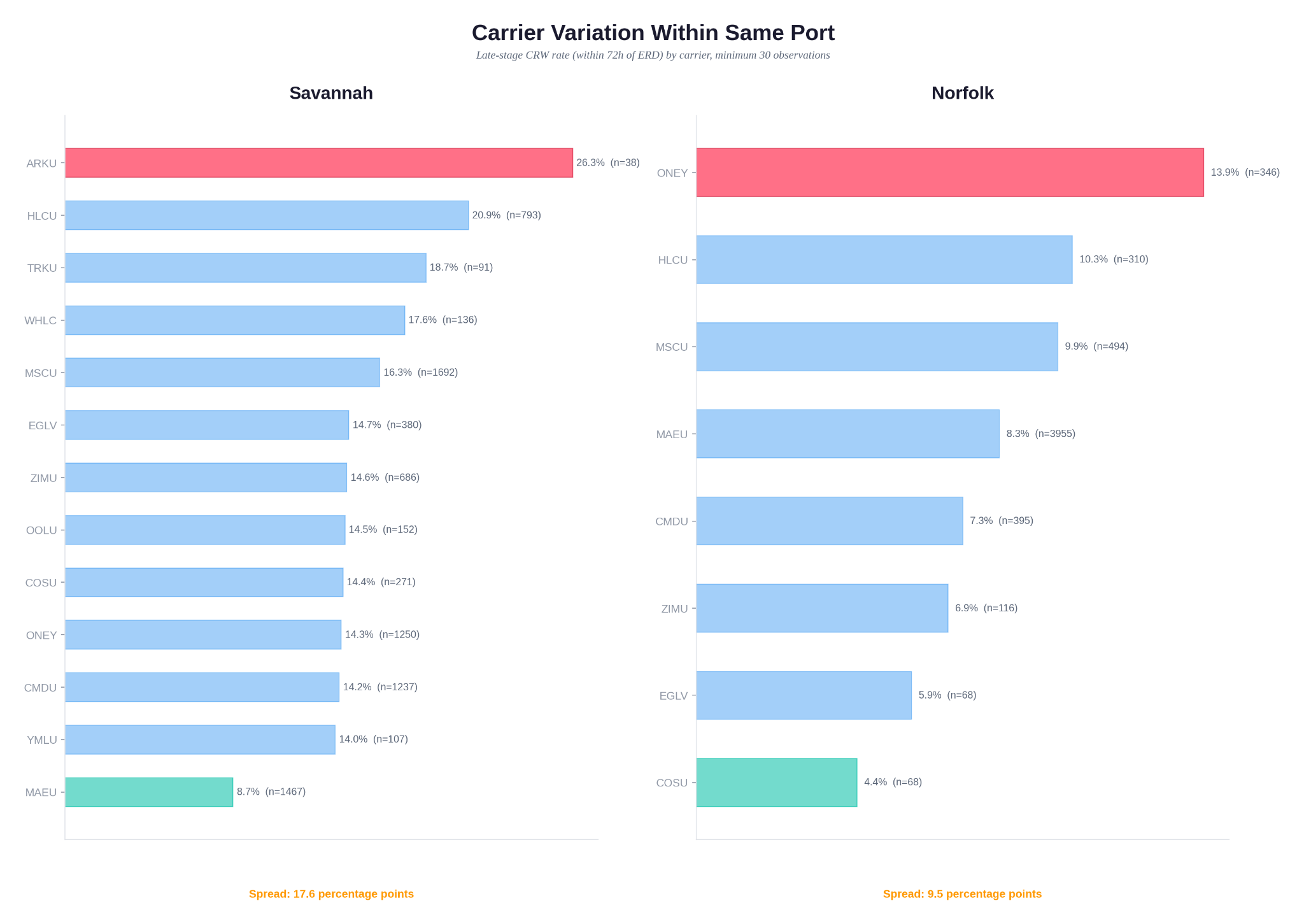
Planning rules must reflect that reality.

Figure 8 - Roll-Level Exposure per 100 Shipments by Gateway

VI. Why “Only 1 in 100” Is Misleading

If you focus only on irreversible roll-level loss, structural volatility appears small.

But the real operational cost is:

• 78 shipments that move
• 29 shipments that demand adjustment
• 20-40+ hours of labor per 100 shipments
• Compressed decision windows that reduce margin for error

Structural volatility is not catastrophic.

It is cumulative.

It is repetitive.

It is time-intensive.

It is the background tax on export operations.

The roll is not the main story.

The labor is.

Figure 9 - The Concentration Cascade

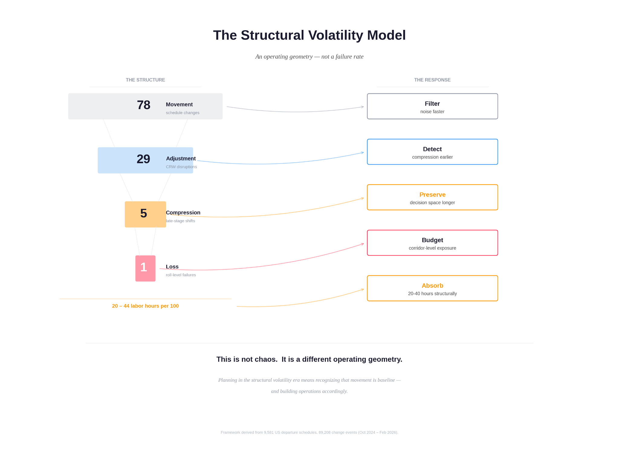
VII. Planning in the Structural Volatility Era

Planning now requires acknowledging:

• Movement is baseline - 78 per 100
• Adjustment is structural - 29 per 100
• Late-stage compression concentrates risk - 5 per 100
• Roll-level loss is measurable - ~1 per 100 in aggregate
• Labor cost is material - 20-40+ hours per 100

This is not chaos.

It is a different operating geometry.

The objective is not to stop windows from moving.

It is to:

• Filter noise faster
• Detect compression earlier
• Preserve decision space longer
• Budget corridor-level exposure
• Design systems that absorb 20-40 labor hours per 100 shipments

The boundary is ERD to CY Cut.

The stress accumulates in the 29.

The collapse concentrates in the 5.

The loss appears in the 1.

Planning in the structural volatility era means recognizing that movement is baseline - and building operations accordingly.

Figure 10 - The Structural Volatility Model